Classification analysis

Classification analysis

Classification is a machine learning technique that constructs a model to predict discrete values for each row in your data. These models predict outcomes with values like yes/no, true/false, or binary numerical values. It is recommended that you utilize various classification algorithms for model comparison.

Overview

In Lumenore’s “Do You Know,” the Classification process involves two steps. Initially, you build a model by specifying input and target columns from an uploaded dataset. Once the model is created, it can be applied to another dataset with the same input columns, predicting the target values.

Note: Ensure the schema contains at least two variables for classification analysis.

Steps to perform classification analysis in Lumenore:

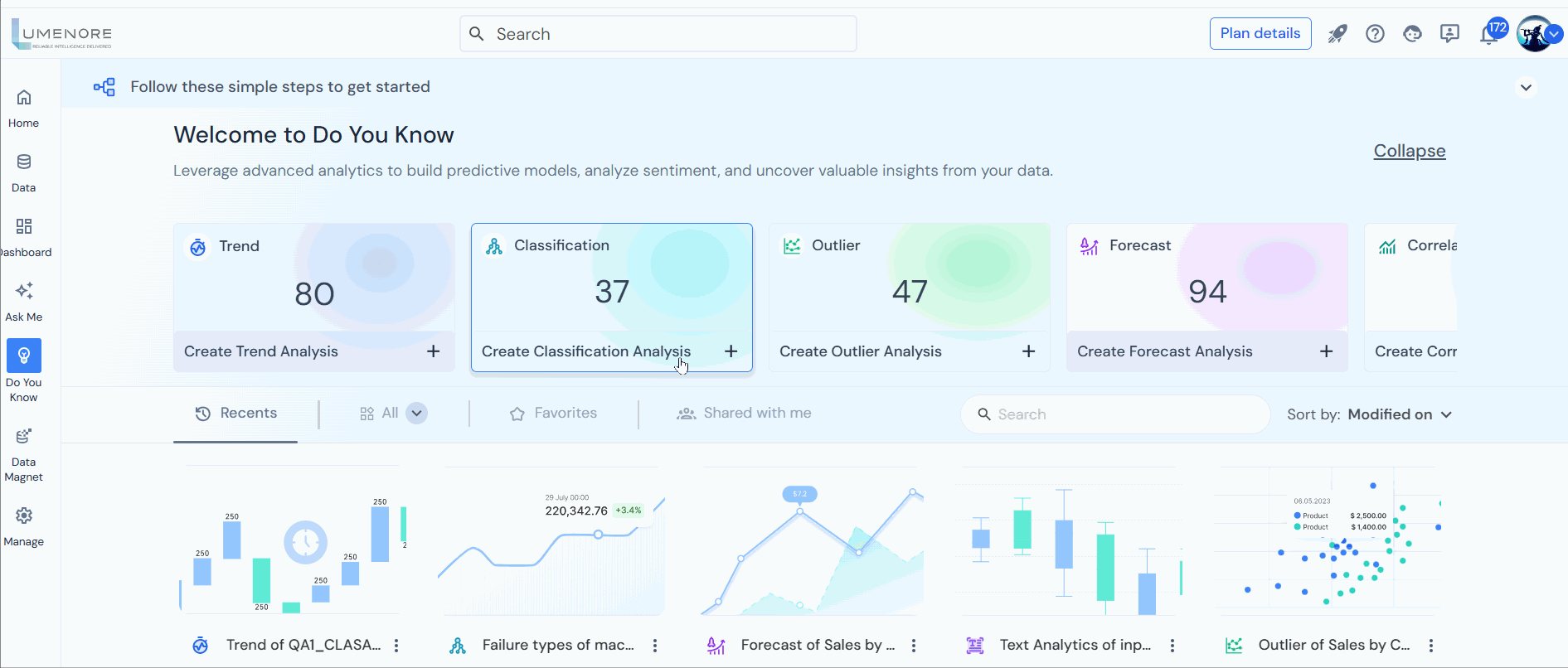
Step 1: After accessing “Do You Know,” select “Classification.”

Step 2: Choose a Schema and click “Next.”

Note: The schema signifies the dataset for analysis. If absent, create one, ensuring prerequisites (A KPI, Date, and Attribute) are met.

Step 3: Select the following to configure:

• Select insight approach: Choose the insight approach, providing two options: “Build a new machine learning model” or “Reuse an existing model.” To create a new model, select the first option. If you’ve previously built a Classification model, choose the second option to generate forecasts using that model.
• Select model: It is deactivated for “Build a new machine learning model” and activated for “Reuse an existing model.”
• Select output variable: Choose the output variable for the classification model. Ensure it comprises precisely two distinct values (a binary variable).
• Select unique identifiers: In this context, the chosen variable(s) will uniquely identify rows and will not be utilized for constructing the model.
• Select input variables: Kindly choose the input variable(s) required for constructing the classification model.
• Algorithm: Choose a classification algorithm to develop your model. Do You Know offers various widely utilized ML algorithms such as Logistic Regression, Decision Tree, Random Forest, and XG Boost.
  • Logistic Regression: Logistic regression is a statistical technique used for binary classification, where the aim is to predict one of two possible outcomes based on input features. This supervised machine learning algorithm estimates the probability that an input belongs to a particular class. The output is a probability value between 0 and 1, where values near 0 represent low probability and those near 1 represent high probability. A threshold, often set at 0.5, classifies data points based on predicted probabilities. Logistic regression is known for its simplicity, interpretability, and scalability to handle large datasets. It can also be extended to solve multi-class classification problems using one-vs-rest or multinomial logistic regression methods.
  • Decision Tree: The decision tree algorithm is employed for classification and regression tasks. It constructs a tree-like structure by recursively dividing the data based on input feature values to make decisions or forecasts. Decision trees are advantageous for their interpretability and ability to handle categorical and continuous features. However, they can be susceptible to overfitting, especially as the tree complexity increases.
  • Random Forest: Random Forest is an ensemble learning technique for classification and regression tasks. It creates an ensemble of decision trees by training each tree on random subsets of the training data and features. This approach introduces randomness into the model, mitigating overfitting, a common problem with individual decision trees.
  • XG Boost: XGBoost, short for eXtreme Gradient Boosting, is a robust gradient boosting framework popular for its performance in machine learning competitions and real-world applications. It employs an optimized implementation of gradient boosting, sequentially constructing decision tree ensembles. Each subsequent tree aims to rectify the mistakes of its predecessor. XGBoost focuses on optimized tree construction and regularization techniques to prevent overfitting.
• Split ratio: The split ratio train-test method assesses a model’s performance by dividing the data into two sets: training and testing sets. The training set educates the model, while the testing set evaluates its performance.

Note: An 80:20 split implies that 80% of the data is allocated for training, and the remaining 20% is reserved for testing. The split ratio is typically determined based on the dataset’s size and the model’s complexity. This approach offers a significant advantage by allowing the model to train and validate on distinct datasets. This helps prevent overfitting, a scenario where a model excessively fits the training data, resulting in poor performance when presented with new, unseen data.

• Do you want to add filters? Optionally add filters.
• Advance settings (Optional): High cardinality in a column signifies that the column encompasses numerous distinct values, which isn’t favourable for constructing classification models.

Conversely, low-variance columns are also unsuitable for model buildings. Therefore, these settings enable users to exclude such columns from the dataset.

Click “Next.”

Case 1: Selecting to build a new machine-learning model

Step 4: Users can tailor the insights narrative, outlining all the variables in crafting the insight. Then, click on “Save.”

Note: If you wish to apply a filter, a window will appear for creating filters. As shown in the Trend Analysis, establish filters by groups or conditions as needed.

Step 5: Name the insight for future access (default suggestion provided) and save it.

Step 6: A new window appears; click “Execute Now” to generate insights.

Upon initiation of execution, the system will undergo four background processes. You can also terminate the execution at any point before its completion.

To enhance comprehension, we’ve developed a classification model to show the impact of input variables on the model’s performance.

Following the classification analysis conducted using the created model, users can leverage the same model to generate a forecast for similar data.

Case 2- Re-use already available model

Step 1: After choosing schema, select “Reuse an existing model” in the insight approach, then select the previously created model for classification.

Click “Next.”

Step 2: Users can tailor the insights narrative, outlining all the variables in crafting the insight. Then, click on “Save.

Step 3: Name the insight for future access (default suggestion provided) and save it.

Step 4: A new window appears; click “Execute Now” to generate insights.

The forecast analysis insight in classification displays the forecast on classified variables.